An introduction to the quantum world
Reading time: 20 minutes
Contents
If you want to drive a car, do you need to understand how its engine works? Of course, you don’t! In a similar vein, you don’t need to know the details of quantum physics to read the rest of this book. So, feel free to skip this chapter.
Nevertheless, we know that most people want to have some conceptual intuition about what quantum mechanics really is. It is not natural to leave one of the most used words in this book as an abstract concept, and it might be hard for the human brain to proceed without at least seeing some examples.
Here is my best attempt to explain quantum mechanics in accessible terms. Proceed with caution, as things will almost certainly get confusing from here.
What is quantum?
Quantum physics or quantum mechanics is the theory that describes the tiniest particles, such as electrons, atoms, and small molecules. The theory is meant to describe the fundamental laws of nature using a set of mathematical equations, allowing us to predict cause and effect at the scale of nanometres. It answers questions like ‘What happens when I bring two electrons close together?’ or ‘Will these two substances undergo a chemical reaction?’. You can contrast quantum mechanics to Newton’s classical physics, which we learned in high school. The classical theory works great for objects the size of a building or a football but becomes inaccurate at much smaller scales. Quantum is, in a sense, a refinement of classical physics: the theories are effectively identical when applied to a coffee mug, but the more difficult quantum theory is needed to describe very small things.
Some examples of systems where quantum could play a role are:
-
Atoms and the electrons that orbit around them.
-
Flows of electricity in microscopic (nano-scale) wires and chips.
-
Photons, the particles out of which light is made.
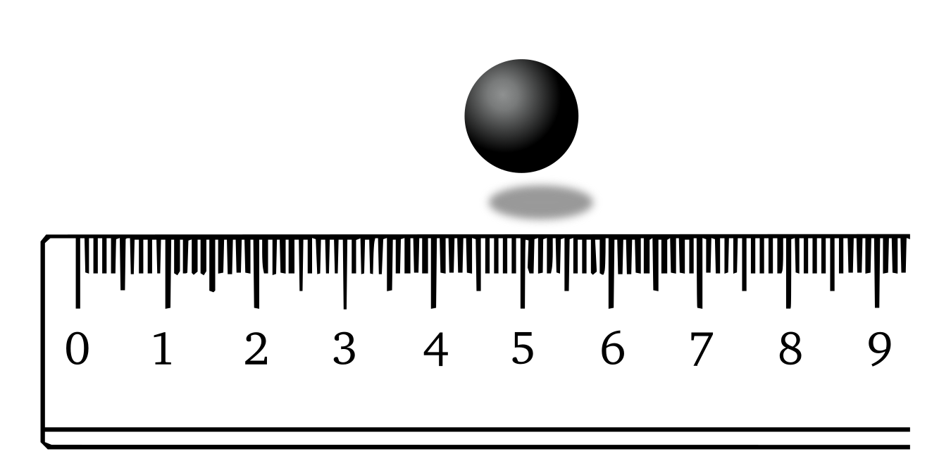
We are going to need some physics jargon to proceed. We like to use the word ‘state’, which is a complete description of all the physical properties of the world at one instance: the locations of all the different particles, their velocities, how much they rotate, etc. Usually, the entire universe is too big to study, so we often simplify our world to a single, isolated particle or to a limited piece of computer memory. Let’s imagine a bare particle in an otherwise empty world. We may be interested in its location, which we’ll call \(x\). For example, the world might look something like the image below, which can be described by a very simple state: \(x = 5\) (the ruler is just virtual).
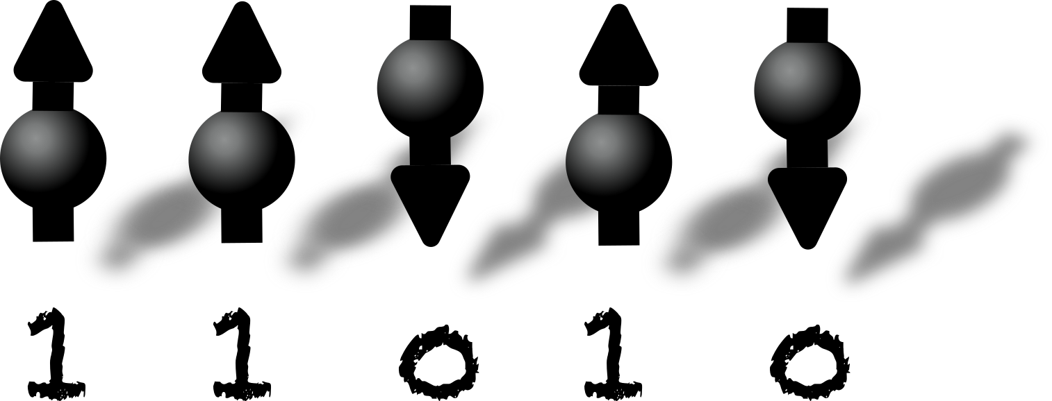
In the spirit of computing, we might look at a ‘bit’ that stores information. Think of it as a tiny magnet that can either point ‘up’ (1) or ‘down’ (0). The state of a piece of memory is easy to describe, simply by expressing the bit values one by one. For example: 11010.
Importantly, the state of the world can change over time. We will often care about the state of the world at a certain moment, for example, at the beginning of a computation or at the end of it.
Four surprising phenomena
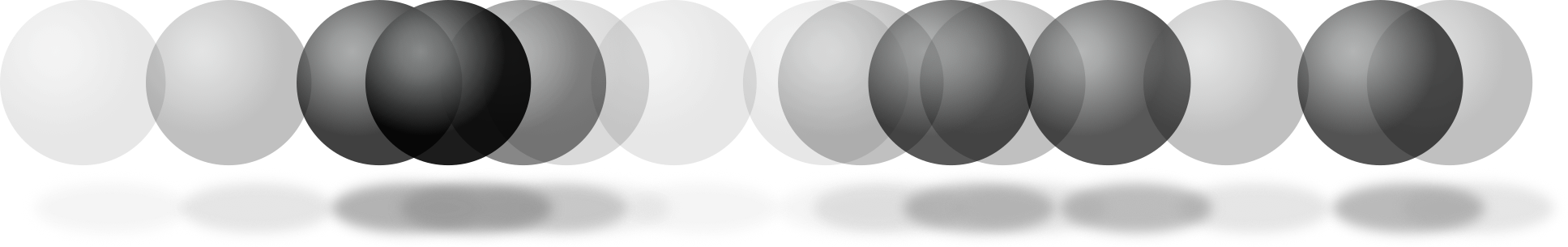
The most iconic quantum phenomenon is superposition. Think about any property that we can (classically) measure, such as the position of a particle or the value of a bit on a hard drive (0 or 1). In quantum mechanics, many different measurement outcomes can be somewhat ‘true’ at the same time: a particle can be in multiple positions at once, or a bit could be 0 and 1 simultaneously. When we say ‘at the same time’ we mean that, to predict any cause and effect, we need to keep track of all these possibilities. To illustrate a superposition, I sometimes picture a quantum particle splitting into many opaque copies of itself, spread out over space, where the degree of transparency determines how likely the particle is to be found there: the darker it is, the more presence it has at that location.
To throw in some more examples of superpositions: an electron can move at a velocity of 10 m/s and 100 m/s at the same time (which obviously also leads to a superposition in its location). More relevant for us: a computer memory might store the numbers 5 and 11 ‘simultaneously’ or even 46 different Microsoft Excel spreadsheets ‘at once’. An important building block to make this all work is the qubit, which is any kind of hardware that can store bit values 0 and 1, and any possible superposition of these two. If we have a bunch of qubits together, we’ll call it a quantum memory.
Let us illustrate the weirdness of superpositions with an example where the 46 spreadsheets each take 1 megabit (Mb) to store. A regular, classical hard drive would allocate the first Mb to a first spreadsheet, then another Mb to store the second, and so forth. In total, it would use 46 Mb. The quantum memory has an additional option to store the spreadsheets in superposition: using the qubit-equivalent of just 1Mb (one million qubits) it would encode all the data in just that limited amount of memory. Whereas 1 Mb of classical memory can fit just one spreadsheet, a quantum memory of 1 Mb can represent several of them, all thanks to the unique properties of quantum physics. However, as we’ll see later, there is a catch to storing all that data so compactly.
How can you possibly describe a world where particles and computer memories are in superposition? For now, let’s focus on an isolated particle. We specify its state using a lengthy list, where for each possible position, we store a number called the amplitude, which is related to how likely the particle is to be found at that location. In other words, the state describes precisely to what extent a particle is at position \(x = 0\), to what extent at position \(x = 1\), and so forth, for every possible location that the particle can be at. And indeed, this list could be infinitely long! Luckily, when dealing with computers, we work with simpler objects. A quantum bit needs just two amplitudes, which denote the extent to which the bit is ‘0’ or ‘1’, respectively.
The amplitudes used to describe quantum states feel somewhat analogous to probabilities, which can similarly tell us the likelihood that, for example, a particle can be found at a particular location. However, there is a fundamental difference. Probabilities in the classical world help us deal with information we don’t have: surely, the particle is already at some location, but perhaps we just don’t know which location yet. Quantum mechanics is different. Even if we know every tiny detail about the location of a particle, we still need to describe it as a superposition. Fundamentally, the location is not determined yet. Hence, there is literally no better way to describe the particle than by tracking this convoluted superposition. Amplitudes are also more finicky to deal with than probabilities because these numbers can become negative (and for math experts, they can even be complex numbers).
The second weird phenomenon is how quantum measurements work. Why do we never observe an electron at two places at the same time? Why do I never find a car both moving and standing still? In quantum mechanics, as soon as we measure the location of a particle, it instantly jumps to a single location at random – making its location fully determined. Similarly, when we measure a qubit, it jumps to either ‘0’ or ‘1’. When we measure the data in a quantum memory, we may find any one of the 46 spreadsheets that were stored. A measurement essentially changes a system into a normal, classical state.
The effect of a measurement is intrinsically random (and hence, our world is not deterministic!). But this doesn’t imply that we cannot understand quantum mechanics. We can calculate the probabilities of measurement outcomes with incredible precision as long as we know the state before the measurement.
It is important to note that we cannot learn anything about the world without measuring – it is our only way to obtain data about physical objects. Any observation, even a slight peek at our system, is a measurement in quantum mechanics. Additionally, measurements are destructive in the sense that they change the state of the world. We fundamentally cannot ‘look’ at a particle without disturbing it. In fact, measurements delete all the rich data encoded in a superposition! If a particle was initially at position \(x = 0\),\(\ x = 3\ \)and \(x = 10,\) all simultaneously, then upon measurement, it jumps to one of these three options. To give you a bit of jargon, we call this instantaneous change a ‘collapse.’ From that moment, it is 100% at a fixed location: if, at first, we measure the particle to be at \(x = 3\), then any subsequent measurement will give the same result, until some other force moves it again. In the context of a quantum computation, this means that we should carefully choose when we perform any measurements – we cannot just peek at the data at any moment we like, or we risk disturbing a superposition.
This also means that a single piece of quantum memory cannot store an immense number of spreadsheets at the same time – at least, you wouldn’t be able to retrieve each of them. To store 15 Mb worth of classical data, we need 15 Mb worth of qubits. Hence, quantum computers are not particularly useful for storing classical data.
The fact that a measurement changes the state of the world poses a serious problem for the engineers who are building quantum computers. No matter what material we construct our qubits from, they will surely interact with other nearby particles, and some of these interactions could act like destructive measurements. We call this effect decoherence, and, as we will see later, this forms one of the core challenges to large-scale quantum computation.
At this point, quantum data doesn’t seem particularly useful. Why would we want to deal with superpositions if they lead to all this uncertainty? The important advantage stems from the way in which a quantum computer can process quantum data. Using quantum mechanics, a device can manipulate data in ways that a classical computer could never do.
That leads us to the third unique phenomenon. A quantum computer can manipulate the data it stores using so-called quantum gates, or simply ‘gates’ for short. These are rapid bursts of some physical forces that change the state of one or more qubits. They can turn a classical-looking state into a quantum superposition or vice versa. They can act like logical operations, like the AND and OR gates that are used in classical electronics, but also like new quantum logic that has no classical counterpart.
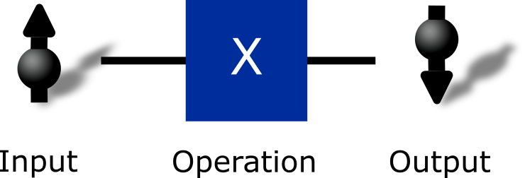
From a functional perspective, a quantum gate takes one or more qubits as input, changes their internal state, and then outputs the same number of qubits (with their altered states). In other words, the number of physical objects remains unchanged, but the overall state changes. As an example, you may think of our prototypical magnet that was initially pointing ‘up’, but a quantum gate might flip this to ‘down’. There are many such gates possible, each having a different effect on their input. We like to give them names in capital letters, such as X, Z, H, and CX. Importantly, a quantum gate is deterministic, meaning that its input-output behaviour is always the same, as opposed to the quantum measurements we saw earlier.
The canonical way to describe a quantum computer program is by defining a sequence of quantum gates, where for each gate, we also indicate what qubits are supposed to be the gate’s input. At the end of the computation, we measure all qubits. An example of such a program, using the standard Quantum Assembly (QASM) language, is given below.
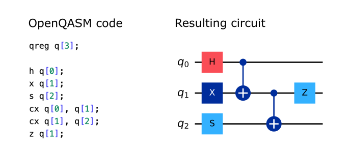
Together, these steps can be graphically displayed in a quantum circuit, as shown here on the right. Quantum circuits represent each qubit with a horizontal line and indicate time flowing from left to right. Whenever a box with a letter is displayed over a qubit line, then the corresponding gate should be applied. This isn’t unlike the way we read sheet music! You may notice that sometimes, two or more gates can be performed in parallel as long as they act on different qubits.
When we run a circuit on an actual quantum computer, the final measurements lead to probabilistic outcomes. We get to see a bunch of ones and zeroes: one classical bit for each qubit. If the circuit is a good quantum algorithm, then, with high probability, these classical bits will tell us the answer we are looking for. But even then, we might need to redo the computation a few times and take (for example) the most common result as our final answer.
If you are completely confused at this point, you are not alone. The whole business of quantum superposition and quantum operations is incredibly complex and is not something you could possibly master after reading a few pages. Scientists who have studied the subject for many years are still frequently baffled by deceptive paradoxes and counter-intuitive phenomena. On the other hand, we hope that the functionality of quantum circuits makes some sense: we define a list of instructions and feed them into a machine that can execute them. We don’t have to know precisely what’s going on under the hood!
There is one remaining quantum phenomenon to cover – one that comes with a mysterious flair surrounding it. We’re talking about quantum entanglement, which we’ll describe using the following example.
Imagine that we have two qubits, which we can transport independently from each other without disturbing the data they store. Together, the qubits can represent the states 00, 01, 10, or 11, or any superposition of these. According to quantum mechanics, we can create a very specific state where the pair of qubits is simultaneously 00 and 11. Now, imagine that computer scientist Alice grabs one of the qubits, takes it on her rocket ship, and flies it all the way to the dwarf planet Pluto. The other qubit remains on Earth in the hands of physicist Bob. Upon arriving on Pluto, Alice measures her qubit and finds outcome ‘1’. A deep question is: what do we now know about Bob’s qubit?
Since the only possible measurement outcomes were 00 and 11, the other qubit can only be measured as ‘1’ from now onwards. It essentially collapses to be 100% in the state ‘1’. But how could the Earth-based qubit possibly know that a measurement occurred on Pluto? What mechanism made it collapse? According to Einstein’s theory of relativity, information cannot travel faster than the speed of light, which translates into a few hours between Earth and Pluto. Nevertheless, measuring the qubits in two faraway locations will always give a consistent result, even when the two qubits are measured at exactly the same time.
This paradox reveals, once again, how confusing quantum mechanics can be. However, the story above is perfectly consistent with both quantum mechanics and the theory of relativity. The core principle is that no information can be sent faster than light between Alice and Bob. For example, can you see why Bob has no way of detecting when Alice performs her measurement just by looking at his entangled qubit? In the most common interpretation of quantum mechanics, the Earth qubit does indeed change its state instantaneously when Alice measures her qubit, although there is no way to exploit this effect for fast messaging.
More generally, entanglement is the phenomenon where two or more faraway qubits can have correlated measurement outcomes that are classically impossible. There is a fascinating further discussion about the philosophy behind entanglement, but we’ll leave that to other sources. What matters to us is that entanglement leads to new functionalities that we can exploit. We will discover what these are in the chapter on quantum networks.
So, there you have it: four surprising phenomena you may hear frequently in quantum technology conversations. To summarise:
-
Superposition: the phenomenon where a qubit is both 0 and 1 at the same time.
-
Quantum measurement: measuring a quantum memory destroys superposition. The result we obtain is probabilistic.
-
Quantum gates: deterministic changes to the state of qubits, which generalise classical logic gates like OR, AND, NOT. A list of several quantum gates (together with the qubits they act on) forms a quantum circuit.
-
Entanglement: qubits separated over a long distance can still share unique properties.
What does a quantum computer look like?
Most large-scale computing today happens in data centres, where we don’t care much about the specifics of the devices that do our calculations. We also expect that future quantum computers will mostly be tucked away in the ‘cloud’, making their appearance and inner workings largely irrelevant to most users. However, for this optional chapter, we can take the opportunity to view what today’s cutting-edge hardware looks like. There are many different ways to build a quantum computer, each based on distinct physical systems and principles. Here, we describe the example of so-called superconducting qubits, a relatively mature platform used by companies like IBM, Google, and Rigetti and several academic institutes. Research institute QuTech in Delft, the Netherlands, was kind enough to provide photos that allow us to look inside their labs. We will see that only a tiny part of the computer is actually ‘quantum’, whereas most of the machine consists of classical machinery that’s required to keep the computer working.

A quantum chip. Photo credits: Marc Blommaert for QuTech.
The real quantum magic happens on a chip, not unlike the computer chips used in your laptop or phone. The qubits are formed by tiny electronic circuits where the flow of electrical current is restricted to just one out of two states: the ‘bit’ states 0 and 1. Since this is a quantum system, the current can also be in a superposition – picture all the electrons in the wire participating both in flow ‘0’ and flow ‘1’ simultaneously! This only works when the chip is cooled down to unimaginably low temperatures, down to around 10 millikelvin – a hundredth of a degree above absolute zero. At these temperatures, the electronic circuits become superconducting, such that an initial current can flow indefinitely. This is important because any damping of the current would cause unwanted disturbance to the qubit state.
The temperature constraint is why the quantum chip is placed in a massive dilution refrigerator, a cylinder of about half a metre in diameter and over a metre tall, which specialises in keeping the quantum chip cool. In the future, larger quantum computers may need even bigger fridges or combine several of these close together. Deeper parts of the fridge have increasingly low temperatures, allowing us to cool in stages. An example could be to cool a first environment to 35 Kelvin (-283 °Celsius or -396.7 °Fahrenheit), followed by subsequent stages to ~3K, 900mK, 100mK, until the final stage of ~10mK is reached.
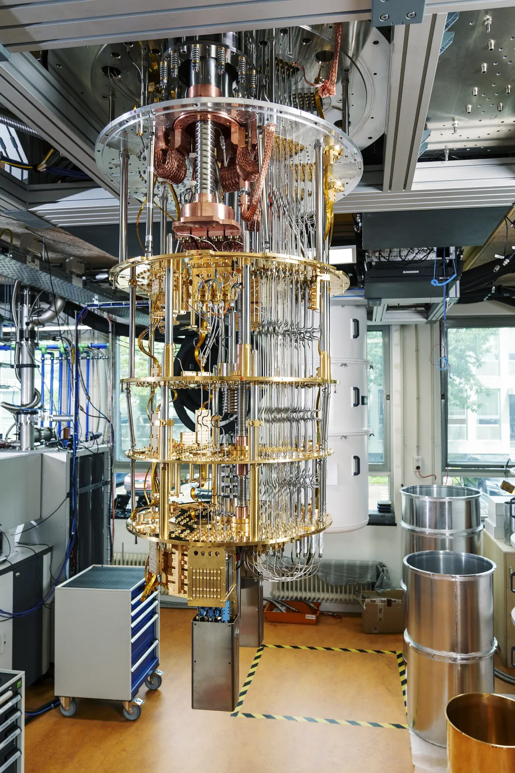
The interior of a dilution fridge, as used for superconducting quantum computers. Photo credits: Marc Blommaert for QuTech.
Engineers typically suspend the fridge on the ceiling so that the higher temperatures are on top, and the ultracold quantum chip is placed at the very bottom. The internals are shaped accordingly: several layers of gold disks are hung below one another, one disk for each temperature zone. A large number of wires run between the disks, transporting signals between the ceiling and the lowermost areas. The whole structure forms the iconic metal chandelier that you often see in images, although it would all be covered by a boring metal case when the fridge is in operation.
To make the qubits do something useful, like executing a quantum gate or performing a measurement, we need to send signals into the chip. Just like with classical computers, a ‘signal’ is a voltage difference between two or more wires. Some voltages remain constant over time, others oscillate at microwave frequencies. Having a larger number of wires can lead to more precise quantum gates, but extensive wiring also leads to two fundamental challenges. Firstly, we currently need around 2–4 wires to control a single qubit, which is problematic when we scale to millions of qubits – it’s impossible to connect that many wires to a tiny chip. We’ll need to find multiplexing solutions, where a single wire can serve multiple qubits at once. Secondly, wires connect the ultracold chip to other hardware that sits at room temperature, forming a channel for heat and noise to enter. The dilution fridge circumvents this by incrementally cooling and damping the signals as they travel through the different layers of the fridge, but it can only handle so many cables.
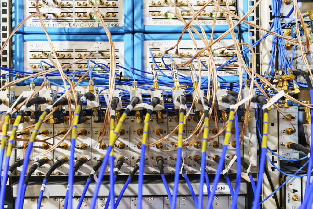
A stack of classical control electronics used to generate and measure electronic signals. Photo credits: Marc Blommaert for QuTech.
Besides the large chandelier, an array of specialised control electronics is needed to produce the necessary electronic pulses and to carefully read out the tiny signals that qubits produce when we measure them. These devices sit in one or multiple electronics racks, each half a metre wide and nearly two metres tall, similar to the ones you’ll find in a typical data centre. Ironically, the actual quantum software can be written on a simple laptop, from where the instructions are passed to the control electronics to run a quantum circuit.
The state of today’s quantum hardware is reminiscent of early computers in the 1940s and 1950s, which similarly occupied entire rooms and required several engineers for all kinds of laborious manual maintenance tasks. Moreover, the dilution fridges are particularly noisy – to the extent that those who operate them ideally do this from a different room – and they are fairly power-hungry. The quantum computer described above consumes around 25 kW, comparable to driving an electric car. Fortunately, we have good reasons to believe that, over the comings decades, quantum computers will become increasingly compact, efficient, powerful, and dependable, much like their classical cousins did.
Further reading
If you’d like to know more about the physics and math behind qubits, we recommend the following sources:
-
Quantum Country is a great online textbook about Quantum Computing by Andy Matuschak and Michael Nielsen.
-
QuTech Academy’s School of Quantum explains a broad range of quantum topics using short videos.
-
(YouTube) A video tour that looks inside IBM’s superconducting quantum computer.s